Chapter 6¶

Incompressible turbulent mean flow¶

Turbulent flows are governed by the Navier-Stokes equations. However,

there are no simplifications possible by dimensional analysis or through similarity solutions,
no exact definition is known for turbulence,
turbulent flows are not very well understood.

Turbulent flows are usually defined by listing their most characteristic properties. Here is what we know

Turbulence is a flow property and not a fluid property.
Turbulence is always three-dimensional in space and transient. There is no such thing as two-dimensional turbulence.
Turbulence is irregular, with seemingly random and chaotic motion. However, there is order to the chaos. The flow satisfies the Navier-Stokes equations, so it is apparently deterministic. Still, N-S are extremely sensitive to initial and boundary conditions (the butterfly-effect). The slightest perturbations in initial or boundary conditions leads to a completely different solution. Thus, turbulence is stochastic even though the Navier-Stokes equations are deterministic.
Turbulent flows consist to a great deal of vortices and vorticity. Vortex stretching and tilting are 3-dimensional phenomena that characterize turbulent flows and these processes can not happen in 2D. If a vortex tube is stretched it must increase its angular velocity to conserve angular momentum. This can only happen in 3D. In 2D vorticity is (unphysically) a conserved quantity.
The vortices come in a range of scales. The size of the largest vortices (the largest scales) is determined by the geometry of the flow, whereas the size of the smallest vortices (the smallest scales) is determined by viscosity.
The energy cascade. Energy is introduced into the flow on the largest scales and dissipated on the smallest. Dissipation \(\varepsilon\) of kinetic energy is defined as

\[ \varepsilon = \mu \boldsymbol{s} : \boldsymbol{s}, \quad {\mathrm{where\,\, strain }}\quad \boldsymbol{s} = 0.5\left( \nabla \boldsymbol{u} + \nabla \boldsymbol{u}^T \right) \]

The strain increases dramatically towards the center of a vortex tube leading to higher dissipation rates in this region.
Turbulence occur at high Reynolds numbers. The normalized momentum equation reads

\[ \frac{\partial \boldsymbol{u}}{\partial t} + (\boldsymbol{u} \cdot \nabla)\boldsymbol{u} = -\nabla p + \frac{1}{Re} \nabla ^2 \boldsymbol{u} + \boldsymbol{f}. \]

Diffusion is stabilizing as it tends to smear out all gradients. Briefly, perturbations (disturbances) to the flow are amplified by convection and dampened by viscosity. If the Reynolds number is large, then diffusion is small and convection dominates, leading to unstable turbulent flows. If the Reynolds number is small then viscosity dominates and perturbations are killed before they can trigger turbulence.

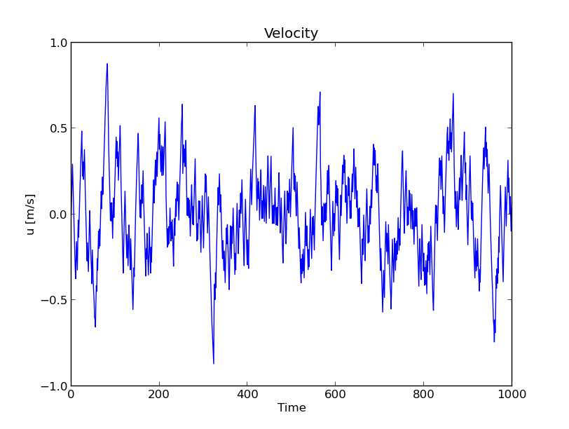
Fig. 5 Figure shows 1000 instantaneous measurements of one chaotic velocity component.¶

Engineers need to be able to predict the behaviour of turbulent flows. However, in a turbulent flow the velocity \(\boldsymbol{u}(\boldsymbol{x}, t)\) and pressure \(p(\boldsymbol{x}, t)\) should really be considered as random variables. In other words, at any point in space and time we will not be able to predict the exact value of velocity or pressure. We can, however, predict the statistical properties of these random variables. This is usually accomplished using ensemble averages or Reynolds averaging.

Consider first a turbulent flow that is statistically steady, i.e., the statistical properties of the flow are independent of time. This happens, e.g., for a plane channel flow or a straight pipe flow where the applied pressure gradient (the driving force) is held constant. As previously stated, in a turbulent flow the velocity vector \(\boldsymbol{u}(\boldsymbol{x}, t)\) can be considered a random variable. If you stand in the same spot inside the statistically steady turbulent flow and measure one velocity component, then the signal will look a lot like Gaussian noise, as can be seen in Fig. 5.

The arithmetic mean of the velocity over these samples can computed as

\[ \left<u\right>(\boldsymbol{x}) = \frac{1}{N} \sum_{i=1}^N u(\boldsymbol{x}, t_i)\]

where \(u(\boldsymbol{x}, t_i)\) is the velocity at time \(t_i\) and \(N=1000\) for the turbulent series shown. If the sampling is done in discrete intervals of time \(\triangle t\), then \(t_i = i\triangle t\). Furthermore, if the samples are taken at sufficiently long time intervals such that \(u(\boldsymbol{x}, t_i)\) is uncorrelated with \(u(\boldsymbol{x}, t_i+\triangle t)\) then we talk about an ensemble average as

\[ \overline{u}(\boldsymbol{x}) = \lim_{N\rightarrow \infty} \frac{1}{N} \sum_{i=1}^N u(\boldsymbol{x}, t_i).\]

By multiplying through by \(\triangle t\) in both numerator and denominator the ensemble average can also be rewritten as

\[\begin{split}\begin{aligned} \overline{u}(\boldsymbol{x}) &= \lim_{N\rightarrow \infty} \frac{1}{N\triangle t} \sum_{i=1}^N u(\boldsymbol{x}, t_i) \triangle t, \\ &\approx \frac{1}{T} \int_0^{T} u(\boldsymbol{x}, t) \mathrm{d} t, \end{aligned}\end{split}\]

where \(T=N\triangle t\) is the total sampling time, which typically needs to be larger than the largest timescales of the flow. It can be seen that for a statistically steady flow the ensemble average corresponds to the time average.

For a more general turbulent flow where the statistics can change in time more care needs to be taken in defining the ensemble average because the random variable \({u}(\boldsymbol{x}, t)\) will in general be statistically different from the random variable \({u}(\boldsymbol{x}, t+\triangle t)\) (e.g., \(\overline{u}(\boldsymbol{x}, t) \neq \overline{u}(\boldsymbol{x}, t+\triangle t)\)). To resolve this, consider flipping a coin. If \(\xi\) is the random variable where head gives \(\xi=1\) and tail \(\xi=0\), then the arithmetic average obviously become

\[ \left< \xi\right> = \frac{1}{N}\sum_{i=1}^N \xi^{(i)}\]

where \(\xi^{(i)}\) is the result of flip \(i\) and as \(N\rightarrow \infty\) we should get \(\left< \xi\right> = 0.5\). Now, if the coins are identical then the arithmetic average is obviously the same if one person flips a coin \(N\) times or \(N\) persons flip one coin one time. This principle is used in defining an ensemble average for turbulent flows. If, instead of sampling the random variable \(u(\boldsymbol{x}, t)\) at \(N\) different time intervals, we run \(N\) identical experiments and sample \(u(\boldsymbol{x}, t)\) at the same time and place in all experiments, then the definition of the ensemble average will be

\[ \overline{u}(\boldsymbol{x}, t) = \lim_{N\rightarrow \infty} \frac{1}{N} \sum_{i=1}^N u^{(i)}(\boldsymbol{x}, t).\]

For a statistically steady flow this will be identical to the time average and the left hand side will not be dependent on time.

By using the ensemble average the instantaneous velocity and pressure may be decomposed into a mean and fluctuating component

(51)¶\[\begin{split}\begin{aligned} \boldsymbol{u}(\boldsymbol{x}, t) &= \overline{\boldsymbol{u}}(\boldsymbol{x}, t) + \boldsymbol{u}'(\boldsymbol{x}, t), \notag \\ p(\boldsymbol{x}, t) &= \overline{p}(\boldsymbol{x}, t) + p'(\boldsymbol{x}, t). \end{aligned}\end{split}\]

Note that both the instantaneous velocity \(\boldsymbol{u}(\boldsymbol{x}, t)\) and the fluctuating velocity \(\boldsymbol{u}'(\boldsymbol{x}, t)\) should be considered as random variables, whereas the mean velocity \(\overline{\boldsymbol{u}}(\boldsymbol{x}, t)\) is deterministic. Consider any random variable decomposed as \(\phi = \overline{\phi} + \phi'\). By definition we have \(\overline{\phi'}=0\). This follows since we can take the average of both sides of Eq. (51) leading to

\[\begin{split}\begin{aligned} \overline{\phi} &= \overline{\overline{\phi} + \phi'},\\ &= \overline{\overline{\phi}} + \overline{\phi'}, \\ &= \overline{\phi} + \overline{\phi'}, \end{aligned}\end{split}\]

that can only be true if \(\overline{\phi'}=0\). (Note that the average of an average is still the average.) Some other useful averaging rules are

\[\begin{split}\begin{aligned} \overline{\phi' \overline{\phi}} &= \overline{\phi'}\, \overline{\phi} = 0,\\ \overline{\phi \overline{\phi}} &= \overline{\phi}\, \overline{\phi}, \\ \overline{\phi \phi} &= \overline{(\overline{\phi} + \phi')(\overline{\phi} + \phi')} = \overline{\phi}^2 + \overline{\phi'\phi'}, \\ \overline{\frac{\partial \phi}{\partial s}} &= \frac{\partial \overline{\phi}}{\partial s}. \end{aligned}\end{split}\]

The last rule follows since the two operations differentiation and averaging commute, i.e., the derivative of an average is the same as the average of a derivative.

Derivation of Reynolds averaged Navier-Stokes (RANS) equations¶

Having defined the average velocity and pressure we are now in a need of equations that can be used to predict them. Equations for any statistical measure can be derived directly by manipulating the Navier-Stokes equations. The equations for \(\overline{\boldsymbol{u}}\) and \(\overline{p}\) are found simply by averaging NS and introducing Eq. (51). Averaging the continuity equation leads to

\[ \overline{\nabla \cdot \boldsymbol{u}} = \nabla \cdot \overline{\boldsymbol{u}} = 0\]

simply because averaging and differentiation commutes. The average of the momentum equation can be written

\[ \overline{\frac{\partial \boldsymbol{u}}{\partial t} + (\boldsymbol{u} \cdot \nabla)\boldsymbol{u} = -\frac{1}{\rho}\nabla p + \nu \nabla ^2 \boldsymbol{u} + \boldsymbol{f}}\]

The density and viscosity are assumed constant. The first term on the left and all terms on the right are averaged by using commutation

\[\begin{split}\begin{aligned} \overline{\frac{\partial \boldsymbol{u}}{\partial t}} &= \frac{\partial \overline{\boldsymbol{u}}}{\partial t}, \\ \overline{\frac{1}{\rho}\nabla p} &= \frac{1}{\rho}\nabla \overline{p}, \\ \overline{\nu \nabla ^2 \boldsymbol{u}} &= \nu \nabla ^2 \overline{\boldsymbol{u}}. \end{aligned}\end{split}\]

This leaves the nonlinear convection term. Using index notation we can take two fast steps using continuity and commutation

\[\begin{split}\begin{aligned} \overline{u_j \frac{\partial u_i}{\partial x_j}} &= \overline{ \frac{\partial u_i u_j}{\partial x_j}} - \cancel{\overline{u_i \frac{\partial u_j}{\partial x_j}}} \\ &= \frac{\partial \overline{u_i u_j}}{\partial x_j}. \end{aligned}\end{split}\]

Inserting now for Eq. (51) we have

\[ \overline{u_i u_j} = \overline{(\overline{u}_i + u_i')(\overline{u}_j + u_j')} = \overline{u}_i \overline{u}_j + \overline{u_i' u_j'}\]

and thus

\[\begin{split}\begin{aligned} \overline{u_j \frac{\partial u_i}{\partial x_j}} &= \frac{\partial \overline{u}_i \overline{u}_j + \overline{u_i' u_j'}}{\partial x_j} \\ &= \overline{u}_j \frac{\partial \overline{u}_i}{\partial x_j} + \frac{\partial \overline{u_i' u_j'}}{\partial x_j} \end{aligned}\end{split}\]

Putting it all together we obtain the Reynolds averaged Navier-Stokes equations

(52)¶\[ \frac{\partial \overline{\boldsymbol{u}}}{\partial t} + (\overline{\boldsymbol{u}} \cdot \nabla)\overline{\boldsymbol{u}} = -\frac{1}{\rho}\nabla \overline{p} + \nu \nabla ^2 \overline{\boldsymbol{u}} - \frac{\partial \overline{u_i' u_j'}}{\partial x_j} + \overline{\boldsymbol{f}},\]

(53)¶\[ \nabla \cdot \overline{\boldsymbol{u}} = 0\]

Derivation of equation for average turbulent kinetic energy¶

The Reynolds averaged Navier-Stokes equations are derived in the previous section. To derive the turbulent kinetic energy equation it can be advantageous to first derive an equation for the fluctuating velocity \(\boldsymbol{u}'\). Such an equation can be derived by subtracting Eq. (52) from the instantaneous momentum equation. All terms are trivial except from the convection

\[\begin{split}\begin{aligned} \frac{\partial \boldsymbol{u} - \overline{\boldsymbol{u}}}{\partial t} + (\boldsymbol{u} \cdot \nabla)\boldsymbol{u} - (\overline{\boldsymbol{u}} \cdot \nabla)\overline{\boldsymbol{u}} &= -\frac{1}{\rho}\nabla (p- \overline{p}) + \nu \nabla ^2 (\boldsymbol{u} - \overline{\boldsymbol{u}}) +\frac{\partial \overline{u_i' u_j'}}{\partial x_j} + \boldsymbol{f} - \overline{\boldsymbol{f}}, \\ \frac{\partial \boldsymbol{u}'}{\partial t} + (\boldsymbol{u} \cdot \nabla)\boldsymbol{u} - (\overline{\boldsymbol{u}} \cdot \nabla)\overline{\boldsymbol{u}} &= -\frac{1}{\rho}\nabla p' + \nu \nabla ^2 \boldsymbol{u}' +\frac{\partial \overline{u_i' u_j'}}{\partial x_j} + \boldsymbol{f}' . \end{aligned}\end{split}\]

The convection terms are manipulated by inserting for \(\boldsymbol{u}\)

\[\begin{split}\begin{aligned} (\boldsymbol{u} \cdot \nabla)\boldsymbol{u} - (\overline{\boldsymbol{u}} \cdot \nabla)\overline{\boldsymbol{u}} &= ((\overline{\boldsymbol{u}}+\boldsymbol{u}') \cdot \nabla)(\overline{\boldsymbol{u}}+\boldsymbol{u}') - (\overline{\boldsymbol{u}} \cdot \nabla)\overline{\boldsymbol{u}}, \\ &= (\overline{\boldsymbol{u}} \cdot \nabla) \boldsymbol{u}' + (\boldsymbol{u}' \cdot \nabla) (\overline{\boldsymbol{u}}+\boldsymbol{u}' ), \end{aligned}\end{split}\]

which gives us the final equation for the fluctuating velocity component

(54)¶\[ \frac{\partial \boldsymbol{u}'}{\partial t} + (\overline{\boldsymbol{u}} \cdot \nabla) \boldsymbol{u}' = -\frac{1}{\rho}\nabla p' + \nu \nabla ^2 \boldsymbol{u}' - (\boldsymbol{u}' \cdot \nabla) (\overline{\boldsymbol{u}}+\boldsymbol{u}' ) +\frac{\partial \overline{u_i' u_j'}}{\partial x_j} + \boldsymbol{f}'.\]

Using index notation throughout the equation reads

(55)¶\[ \frac{\partial u_i'}{\partial t} + \overline{u}_j \frac{\partial u_i'}{\partial x_j} = -\frac{1}{\rho}\frac{\partial p'}{\partial x_i} + \nu \frac{\partial^2 u_i'}{\partial x_j \partial x_j} - u_j'\frac{\partial \overline{u}_i}{\partial x_j} - u_j'\frac{\partial u_i'}{\partial x_j} +\frac{\partial \overline{u_i' u_j'}}{\partial x_j} + f_i'.\]

We now want to use this equation to derive transport equations for the Reynolds stresses and the turbulent kinetic energy. The turbulent kinetic energy is \(k = 0.5 \overline{\boldsymbol{u}' \cdot \boldsymbol{u}'} = 0.5 \overline{u_i'u_i'}\). An equation for \(k\) can be obtained by multiplying Eq. (55) with \(u_i'\) and then taking the average of the resulting equation. However, here we will make the derivation of the Reynolds stress \(\overline{u_i'u_j'}\) first, because then we can get the equation for \(\overline{u_i'u_i'}\) simply by taking the trace of the Reynolds stress equation. Start the derivation by multiplying Eq. (55) by \(u_k'\) and then perform an average of the entire resulting equation. For simplicity we neglect the body force \(f_i\)

\[ \overline{ u_k'\left( \frac{\partial u_i'}{\partial t} + \overline{u}_j \frac{\partial u_i'}{\partial x_j} = -\frac{1}{\rho}\frac{\partial p'}{\partial x_i} + \nu \frac{\partial^2 u_i'}{\partial x_j \partial x_j} - u_j'\frac{\partial \overline{u}_i}{\partial x_j} - u_j'\frac{\partial u_i'}{\partial x_j} +\frac{\partial \overline{u_i' u_j'}}{\partial x_j} \right) }.\]

Most terms are trivially manipulated, and the last term on the rhs disappears

\[\overline{ u_k' \frac{\partial u_i'}{\partial t}} + \overline{u}_j \overline{u_k'\frac{\partial u_i'}{\partial x_j}} = -\frac{1}{\rho}\overline{u_k'\frac{\partial p'}{\partial x_i}} + \nu \overline{u_k'\frac{\partial^2 u_i'}{\partial x_j \partial x_j}} - \overline{u_k'u_j'}\frac{\partial \overline{u}_i}{\partial x_j} - \overline{u_k' u_j'\frac{\partial u_i'}{\partial x_j}}.\]

Since both \(k\) and \(i\) are free indices they can be interchanged into another equation

\[\overline{ u_i' \frac{\partial u_k'}{\partial t}} + \overline{u}_j \overline{u_i'\frac{\partial u_k'}{\partial x_j}} = -\frac{1}{\rho}\overline{u_i'\frac{\partial p'}{\partial x_k}} + \nu \overline{u_i'\frac{\partial^2 u_k'}{\partial x_j \partial x_j}} - \overline{u_i'u_j'}\frac{\partial \overline{u}_k}{\partial x_j} - \overline{u_i' u_j'\frac{\partial u_k'}{\partial x_j}}.\]

Noting that, e.g., \(\partial u_i'u_k'/\partial t=u_i'\partial u_k'/\partial t + u_k'\partial u_i'/\partial t\), you should now be able to realize that the sum of the two previous equations will give us an equation for \(\overline{u_i'u_k'}\)

(56)¶\[\begin{split}\begin{aligned} \frac{\partial \overline{ u_i'u_k'}}{\partial t} + \overline{u}_j \frac{\partial\overline{ u_i'u_k'}}{\partial x_j} =& -\frac{1}{\rho}\left( \overline{u_i'\frac{\partial p'}{\partial x_k}} + \overline{u_k'\frac{\partial p'}{\partial x_i}} \right) \notag \\ &+ \nu \left( \overline{u_i'\frac{\partial^2 u_k'}{\partial x_j \partial x_j}} + \overline{u_k'\frac{\partial^2 u_i'}{\partial x_j \partial x_j}} \right) \notag\\ &- \overline{u_i'u_j'}\frac{\partial \overline{u}_k}{\partial x_j} - \overline{u_k'u_j'}\frac{\partial \overline{u}_i}{\partial x_j} \notag \\ &- \overline{u_i' u_j'\frac{\partial u_k'}{\partial x_j}} - \overline{u_k' u_j'\frac{\partial u_i'}{\partial x_j}}. \end{aligned}\end{split}\]

Several terms on the rhs can be further simplified. Using the product rule the pressure terms can alternatively be written as

\[\begin{split}\begin{aligned} \overline{u_i'\frac{\partial p'}{\partial x_k}} + \overline{u_k'\frac{\partial p'}{\partial x_i}} &= \overline{p' \left( \frac{\partial u_i'}{\partial x_k} + \frac{\partial u_k'}{\partial x_i} \right)} + \frac{\partial}{\partial x_j}\left( \overline{p' u_i'}\delta_{kj} + \overline{p' u_k'}\delta_{ij} \right), \\ &= 2 \overline{p' s_{ik}'} + \frac{\partial}{\partial x_j}\left( \overline{p' u_i'}\delta_{kj} + \overline{p' u_k'}\delta_{ij} \right), \end{aligned}\end{split}\]

where

\[s_{ij}' = \frac{1}{2} \left( \frac{\partial u_i'}{\partial x_j} + \frac{\partial u_j'}{\partial x_i}\right)\]

and the notation with the identity tensor is used to enable a divergence form (\(\partial \overline{p'u_i'}/\partial x_k = \partial \overline{p' u_i'} /\partial x_j \delta_{kj}\)). This notation is used to emphasize that the term is conservative, it can neither create nor destroy \(\overline{u_i' u_k'}\), but simply serves to move it around. For this reason the term is often referred to as pressure diffusion.

The two Laplacian terms in Eq. (56) can be simplified using the following identities

\[ u_i'\frac{\partial^2 u_k'}{\partial x_j \partial x_j} = \frac{\partial}{\partial x_j}\left( \frac{\partial u_i'u_k'}{\partial x_j} - u_k'\frac{\partial u_i'}{\partial x_j} \right) - \frac{\partial u_i'}{\partial x_j} \frac{\partial u_k'}{\partial x_j}\]

and

\[ u_k'\frac{\partial^2 u_i'}{\partial x_j \partial x_j} = \frac{\partial}{\partial x_j}\left( u_k' \frac{\partial u_i'}{\partial x_j} \right) - \frac{\partial u_i'}{\partial x_j} \frac{\partial u_k'}{\partial x_j}.\]

Summing up these two equations we get

\[u_i'\frac{\partial^2 u_k'}{\partial x_j \partial x_j} + u_k'\frac{\partial^2 u_i'}{\partial x_j \partial x_j} = \frac{\partial^2 u_i'u_k'}{\partial x_j \partial x_j} - 2 \frac{\partial u_i'}{\partial x_j} \frac{\partial u_k'}{\partial x_j}.\]

Finally, note that due to continuity

\[ u_i' u_j' \frac{\partial u_k'}{\partial x_j} + u_k' u_j' \frac{\partial u_i'}{\partial x_j} = \frac{\partial u_i' u_k' u_j'}{\partial x_j}.\]

Inserting for all the simplifications above we obtain a final form for the Reynolds stress transport equation

(57)¶\[\begin{split}\begin{aligned} \frac{\partial \overline{ u_i'u_k'}}{\partial t} + \overline{u}_j \frac{\partial\overline{ u_i'u_k'}}{\partial x_j} =& -\frac{2\overline{p' s_{ik}'}}{\rho} - \frac{\partial}{\partial x_j}\left( \frac{1}{\rho}(\overline{p' u_i'}\delta_{kj} + \overline{p' u_k'}\delta_{ij}) + \overline{u_i'u_k'u_j'} - \nu \frac{\partial \overline{u_i'u_k'}}{\partial x_j} \right) \notag \\ &- 2 \nu \overline{\frac{\partial u_i'}{\partial x_j} \frac{\partial u_k'}{\partial x_j}} - \overline{u_i'u_j'}\frac{\partial \overline{u}_k}{\partial x_j} - \overline{u_k'u_j'}\frac{\partial \overline{u}_i}{\partial x_j}. \end{aligned}\end{split}\]

This is the same as Eq.~(6-18) in [Whi06]. Note that on the right hand side only the last two terms on the bottom line and the last on the first line are closed since they only contain \(\overline{u_i'u_k'}\) and gradients of the mean velocity. This means that in our ambitious effort to find a closure for \(\overline{u_i'u_k'}\) from first principles we have ended up creating even more problems for our self.

An equation for the turbulent kinetic energy \(k\) can be obtained by contracting the two free indices in Eq. (57) (set index \(k=i\)). A few terms disappear due to continuity (\(s_{ii}'=0\)) and symmetry leading to

(58)¶\[\begin{split}\begin{aligned} \frac{\partial \overline{ u_i'u_i'}}{\partial t} + \overline{u}_j \frac{\partial\overline{ u_i'u_i'}}{\partial x_j} =& - \frac{\partial}{\partial x_j}\left( \frac{2}{\rho}\overline{p' u_i'}\delta_{ij} + \overline{u_i'u_i'u_j'} - \nu \frac{\partial \overline{u_i'u_i'}}{\partial x_j} \right) \notag \\ &- 2 \nu \overline{\frac{\partial u_i'}{\partial x_j} \frac{\partial u_i'}{\partial x_j}} - 2\overline{u_i'u_j'}\frac{\partial \overline{u}_i}{\partial x_j}. \end{aligned}\end{split}\]

If we simplify this further using \(k = 0.5 \overline{u_i'u_i'}\) we obtain

(59)¶\[\begin{split}\begin{aligned} \frac{\partial k}{\partial t} + \overline{u}_j \frac{\partial k}{\partial x_j} =& - \frac{\partial}{\partial x_j}\left( \frac{1}{\rho}\overline{p' u_i'}\delta_{ij} + \frac{1}{2}\overline{u_i'u_i'u_j'} - \nu \frac{\partial k}{\partial x_j} \right) \notag \\ &- \nu \overline{\frac{\partial u_i'}{\partial x_j} \frac{\partial u_i'}{\partial x_j}} - \overline{u_i'u_j'}\frac{\partial \overline{u}_i}{\partial x_j}. \end{aligned}\end{split}\]

Evidently this equation differs in a few places from Eq.~(6-17) in \cite{white06}. However, the difference is merely due to a few rearrangements and we will now derive also a slightly different form more similar to (6-17). Note that the Laplacian term, i.e., the last of the divergence terms on the rhs of Eq. (58), can alternatively be rewritten using the identity

\[ \nu \frac{\partial^2 u_i' u_i' }{\partial x_j \partial x_j} = 4\nu \frac{\partial s_{ij}'u_i'}{\partial x_j} - 2 \nu \frac{\partial u_i'}{\partial x_j} \frac{\partial u_j'}{\partial x_i}.\]

Inserting this into Eq. (58) leads to

\[\begin{split}\begin{aligned} \frac{\partial k}{\partial t} + \overline{u}_j \frac{\partial k}{\partial x_j} =& - \frac{\partial}{\partial x_j}\left( \frac{1}{\rho}\overline{p' u_i'}\delta_{ij} + \frac{1}{2}\overline{u_i'u_i'u_j'} - 2\nu \overline{s_{ij}'u_i'} \right) \\ &- 2\nu \overline{\frac{\partial u_i'}{\partial x_j} s_{ij}'} - \overline{u_i'u_j'}\frac{\partial \overline{u}_i}{\partial x_j}. \end{aligned}\end{split}\]

Furthermore, the velocity deformation tensor can be decomposed as

\[ \frac{\partial u_i'}{\partial x_j} = s_{ij}' + \omega_{ij}',\]

where the anti-symmetric rotation rate tensor \(\omega_{ij}'\) is given as

\[ \omega_{ij}' = \frac{1}{2} \left( \frac{\partial u_i'}{\partial x_j} - \frac{\partial u_j'}{\partial x_i} \right).\]

Since the contraction of a symmetric tensor with an anti-symmetric is identically zero it follows that

\[\begin{split}\begin{aligned} s_{ij}' \frac{\partial u_i'}{\partial x_j} &= s_{ij}'s_{ij}' + s_{ij}'\omega_{ij}' \\ &= s_{ij}'s_{ij}'. \end{aligned}\end{split}\]

The final form of the turbulent kinetic energy equation, which is also the one that is most often used in the literature, is thus

(60)¶\[\begin{split}\begin{aligned} \frac{\partial k}{\partial t} + \overline{u}_j \frac{\partial k}{\partial x_j} =& - \frac{\partial}{\partial x_j}\left( \frac{1}{\rho}\overline{p' u_i'}\delta_{ij} + \frac{1}{2}\overline{u_i'u_i'u_j'} - 2\nu \overline{s_{ij}'u_i'} \right) \notag \\ &- 2\nu \overline{s_{ij}' s_{ij}'} - \overline{u_i'u_j'}\frac{\partial \overline{u}_i}{\partial x_j}. \end{aligned}\end{split}\]

All terms in the turbulent kinetic energy equation have their own physical interpretation

Rate of change of \(k\) due to non-stationary statistics

\[ \frac{\partial k}{\partial t} \]
Rate of change of \(k\) due to convection

\[ \overline{u}_j \frac{\partial k}{\partial x_j} \]
Conservative transport of kinetic energy in an inhomogeneous field due respectively to the pressure fluctuations, the turbulence itself, and the viscous stresses:

\[ \frac{\partial}{\partial x_j}\left( \frac{1}{\rho}\overline{p' u_i'}\delta_{ij} + \frac{1}{2}\overline{u_i'u_i'u_j'} - 2\nu \overline{s_{ij}'u_i'} \right) \]
Rate of production of turbulence kinetic energy from the mean flow (gradient):

\[ \overline{u_i'u_j'}\frac{\partial \overline{u}_i}{\partial x_j} \]
Rate of dissipation of turbulence kinetic energy per unit mass due to viscous stresses:

\[ \varepsilon = 2\nu \overline{s_{ij}' s_{ij}'} \]

Turbulence modelling¶

Turbulence modelling is all about finding suitable closures, or models, for the Reynolds stress tensor. The Reynolds stress tensor is symmetrical

\[ \overline{u_i'u_j'} = \overline{u_j'u_i'}\]

and thus contains 6 unknown quantities. The Reynolds stress is not really a stress, but it is so called because of the way it appears in the mean momentum equation (52). The mean momentum equation can alternatively be rewritten as

(61)¶\[ \rho \left(\frac{\partial \overline{\boldsymbol{u}}}{\partial t} + (\overline{\boldsymbol{u}} \cdot \nabla)\overline{\boldsymbol{u}} \right) = \nabla \cdot \overline{\tau} + \rho\overline{\boldsymbol{f}}, \]

where

\[\overline{\tau}_{ij} = -\overline{p}\delta_{ij} + 2 \mu \overline{S}_{ij} - \rho\overline{u_i'u_j'},\]

is a new term that has dimensions of stress and

\[ \overline{S}_{ij} = \frac{1}{2}\left(\frac{\partial \overline{u}_i}{\partial x_j} + \frac{\partial \overline{u}_j}{\partial x_i} \right).\]

Mathematically then it appears that the total mean stress tensor has been added a third term \(-\rho \overline{u_i'u_j'}\) after the regular pressure and viscous stresses. The term is called a Reynolds “stress”, but it is in fact just the contribution of the fluctuating velocities to the mean nonlinear convection. (Note that \(\rho\) is required for the term to have dimensions of stress.) By stress we usually mean the internal forces that fluid particles exert on each other.

The highest level of RANS modelling is usually considered the second moment closures that solve transport equations for \(\overline{u_i'u_j'}\) directly. Second moment closures are outside the scope of this course.

The by far most commonly used turbulence model is the eddy viscosity (first moment) closure

(62)¶\[ \overline{u_i'u_j'} = -2\nu_T\overline{S}_{ij} + \frac{2}{3}k\delta_{ij},\]

where \(\nu_T\) is a ‘turbulent viscosity’. Turbulence models are usually classified by the number of additional PDE’s that are used to model the turbulent viscosity.

The turbulent viscosity is a parameter of the flow and not the fluid. As mentioned before, one of the most important properties of a turbulent flow is its ability to efficiently mix momentum and scalars, like temperature. Mathematically, the enhanced mixing is manifested through the Reynolds stress and it is through Eq. (62) sought modelled as a diffusion process using \(\nu_T\) as a positive (\(\ge0\)) mixing rate constant. Inserted into the momentum equation the eddy viscosity gives rise to the term

\[ \frac{\partial \overline{u_i'u_j'}}{\partial x_j} = -\frac{\partial }{\partial x_j}\left[ \nu_t \left( \frac{\partial \overline{u}_i}{\partial x_j} + \frac{\partial \overline{u}_j}{\partial x_i} \right) \right] + \frac{2}{3} \frac{\partial k }{\partial x_i},\]

and it can be seen that the first term on the right hand side will lead to enhanced mixing (or diffusion) of \(\overline{u}_i\) as long as \(\nu_T\) is positive.

Having established an algebraic model for the Reynolds stress (62), we have reduced the number of unknowns from 6 to 2 (\(\nu_T\) and \(k\)). We will now discuss the most common strategies for closing the remaining terms.

The turbulent viscosity is by dimensional reasoning the product of a velocityscale \(\tilde{u}\) and a lengthscale \(l\)

\[ \nu_T = \tilde{u} \cdot l,\]

where different interpretations are possible for defining such scales. Remembering that one of the ‘defining’ properties of turbulence is that it contains a range of scales, such a classification into one single velocity- and lengthscale may seem questionable from the very start. Nevertheless, most turbulence models boil down to finding good approximations for these scales, and the modelled scales are then usually interpreted as the largest scales of turbulence. Many different models exist (including multiscale models, which is beside the scope for this course) and sometimes a timescale \(t_k\) is used instead of \(\tilde{u}\), but then the two are related through \(\tilde{u} = l / t_k\).

Turbulence models are usually classified by the number of additional PDEs that are required to establish the proper scales and we will now go through some of the most basic models.

Zero-equation models¶

Zero-equation turbulence models are models that use zero additional PDEs to model the turbulent viscosity. The Mixing length model was the first such turbulence model. For a simple plane shear flow where \(\overline{u}\) is the tangential velocity and \(y\) is the wall normal direction the model reads

(63)¶\[\begin{split}\begin{aligned} \tilde{u} &= l \left|\frac{\mathrm{d} \overline{u}}{\mathrm{d} y} \right|, \notag \\ \nu_T &= l^2 \left|\frac{\mathrm{d} \overline{u}}{\mathrm{d} y}\right|. \end{aligned}\end{split}\]

For a plane shear flow the model is excellent as one may choose

(64)¶\[\begin{split}\begin{aligned} l &\approx y^2, \quad \mathrm{for} \quad y^+ < 5, \notag\\ l &\approx \kappa y, \quad \mathrm{for} \quad 30 < y^+ < 100, \notag \\ l &\approx 1, \quad \mathrm{for} \quad y^+ > 100 \end{aligned}\end{split}\]

where \(\kappa=0.41\) is von Kármán’s constant and \(y\) is the distance to the wall. Further

\[\begin{split}\begin{aligned} v^* &= \sqrt{\nu \frac{\partial \overline{u}}{\partial y}}_{\mathrm{wall}}, \\ y^+ &= \frac{y v^*}{\nu}, \end{aligned}\end{split}\]

are, respectively, the turbulent wall friction velocity and the distance to the wall in normalized ‘wall’ units. A Reynolds number based on the friction velocity, \(Re_{\tau}=L\cdot v^*/\nu\), is often used to characterize flow in turbulent plane shear flows.

Several models exist that merge the three domains in Eq. (64) into one single continuous function. Van Driest provided a model that merged the first two inner layers using

(65)¶\[ l = \kappa y \left(1 - \exp\left( -\frac{y^+}{A}\right) \right),\]

where \(A\) is a constant set to 26 for flat plate flow. This model should be merged with \(l=\mathrm{constant}\) far enough from the wall. Far enough is often chosen when \(l\) from Eq. (65) becomes larger than a factor of the mixing layer thickness \(\delta\). An often used estimate is when \(\kappa y = 0.09\delta\) or \(y = 0.22 \delta\).

The Mixing length model is not a good model for other flows than plane boundary layer flows. For example, in the center of a plane channel the mean velocity gradient is zero due to symmetry (\(\mathrm{d} \overline{u} / \mathrm{d} y = 0\)). The Mixing length model Eq. (63) thus predicts that the turbulent viscosity should be zero in the center of the channel. This is contrary to the experimental observation and intuition, because the turbulent intensity is actually very large in the center.

This flaws of the mixing length model first led to the suggested improvement that the velocityscale should be proportional to the turbulence intensity and not the mean velocity gradient

(66)¶\[ \tilde{u} = \mathrm{const} \cdot \sqrt{k}.\]

The problem now is that this model introduces a new unknown \(k\) that requires modelling (whereas the old model used known quantities \(l\) and \(\overline{u}\)). Thus one additional PDE is required for closure of the turbulent viscosity.

One-equation models¶

Most one-equation turbulence models solves a transport equation for \(k\), the turbulent kinetic energy. The equation for \(k\) has already been derived in previous assignments and it is evident that it contains even more unclosed terms. If we start by rewriting the \(k\)-equation as

(67)¶\[\begin{aligned} \frac{\partial k}{\partial t} + \overline{u}_j \frac{\partial k}{\partial x_j} =& - \frac{\partial T_j}{\partial x_j} \notag + P - \tilde{\varepsilon} \end{aligned}\]

then the terms on the right hand side are

(68)¶\[\begin{split}\begin{aligned} T_j &= \frac{1}{\rho}\overline{p' u_i'}\delta_{ij} + \frac{1}{2}\overline{u_i'u_i'u_j'} - \nu \frac{\partial k}{\partial x_j}, \\ P &= -\overline{u_i'u_j'}\frac{\partial \overline{u}_i}{\partial x_j}, \\ \tilde{\varepsilon} &= \nu \overline{\frac{\partial u_i'}{\partial x_j} \frac{\partial u_i'}{\partial x_j}} . \end{aligned}\end{split}\]

Here \(T_j\) represents turbulent transport, \(P\) is production of turbulent kinetic energy and \(\tilde{\varepsilon}\) is ‘pseudo’-dissipation of turbulent kinetic energy. The production \(P\) is closed since it only contains known quantities like the Reynolds stress and mean velocity gradients. The first two terms of \(T_j\) and \(\tilde{\varepsilon}\) are unknown and require closure. \(\tilde{\varepsilon}\) is called ‘pseudo’-dissipation since the actual dissipation of \(k\) is really \(2\nu\overline{s_{ij}' s_{ij}'}\). The two terms are related through the identity

\[\begin{split}\begin{aligned} 2\nu\overline{s_{ij}' s_{ij}'} &= \nu \overline{\frac{\partial u_i'}{\partial x_j} \frac{\partial u_i'}{\partial x_j}} + \nu \overline{\frac{\partial u_i'}{\partial x_j} \frac{\partial u_j'}{\partial x_i}}, \\ \varepsilon &= \tilde{\varepsilon} + \nu \overline{\frac{\partial u_i'}{\partial x_j} \frac{\partial u_j'}{\partial x_i}}. \end{aligned}\end{split}\]

Since the last term on the rhs is small relative to the first, dissipation and ‘pseudo’-dissipation are similar for most flows.

The turbulent transport term is usually modelled as gradient diffusion

\[ T_j = -\left(\nu + \frac{\nu_t}{\sigma_k} \right) \frac{\partial k}{\partial x_j} ,\]

where \(\sigma_k\) is a constant in the near vicinity of one. Like the name suggests the model enhances diffusion of \(k\) and serves to smooth out the \(k\) field faster than possible simply through regular diffusion. This corresponds well with our knowledge of turbulence as an efficient mixing process.

The ‘pseudo’-dissipation rate scales like

\[ \tilde{\varepsilon} \approx \frac{\tilde{u}^3}{l}.\]

Thus we can find a suitable model for \(\tilde{\varepsilon}\) simply by inserting for Eq. (66)

\[\begin{split}\begin{aligned} \tilde{\varepsilon} &= \frac{(\mathrm{const} \cdot \sqrt{k})^3}{l}, \\ \tilde{\varepsilon} &= \mathrm{const} \cdot \frac{k^{3/2}}{l}, \\ \end{aligned}\end{split}\]

and thus

\[\begin{split} l = \mathrm{const} \cdot \frac{k^{3/2}}{\tilde{\varepsilon}}. \\\end{split}\]

By inserting for the velocity- and lengthscales we get the following model for the turbulent viscosity

\[\begin{split}\begin{aligned} \nu_T &= \mathrm{const} \cdot \sqrt{k} l, \\ \nu_T &= \mathrm{const} \cdot \frac{k^2}{\tilde{\varepsilon}}. \end{aligned}\end{split}\]

A weakness of the model is that it requires the lengthscale \(l\) to be provided from knowledge of the problem under consideration. For this reason one-equation turbulence models are often referred to as being incomplete. One-equation models are popular for systems where the mixing length can be easily specified, like a plane boundary layer or an aeroplane wing.

Two-equation models¶

Two-equation turbulence models introduce an additional PDE for the missing lengthscale. Since two-equation models do not require any parameter (like \(l\)) from previous knowledge of the system, the two-equation models are often referred to as being complete.

The most popular two-equation turbulence models are variations of the \(k-\tilde{\varepsilon}\) model and the \(k-\omega\) model. \(k-\tilde{\varepsilon}\) models solve one PDE for \(k\) and an additional for \(\tilde{\varepsilon}\). Likewise, \(k-\omega\) models solve PDEs for \(k\) and \(\omega\), where \(\omega\approx \tilde{\varepsilon} / k\). If \(k\) and \(\tilde{\varepsilon}\) are known then

\[ l = \frac{k^{3/2}}{\tilde{\varepsilon}}, \quad t_k = \frac{k}{\tilde{\varepsilon}}, \quad \tilde{u} = \frac{l}{t_k} = \sqrt{k}\]

where \(t_k\) is a turbulent timescale. The turbulent viscosity is as before determined by

\[ \nu_T = \mathrm{const} \cdot \tilde{u} \cdot l = \mathrm{const} \cdot \frac{k^2}{\tilde{\varepsilon}}.\]

A transport equation for \(\tilde{\varepsilon}\) can be derived exactly from the Navier-Stokes equations. The resulting equation contains many new unknowns and here we will not go into detail. Instead we will here simply report the entire and closed \(k-\tilde{\varepsilon}\) model with its most common model ‘constants’

(69)¶\[\begin{split}\begin{aligned} \frac{\partial \overline{u}_i}{\partial t} + \overline{u}_j \frac{\partial \overline{u}_i}{\partial x_j} &= \frac{\partial}{\partial x_j}\left[ \left( \nu + \nu_T \right) \left(\frac{\partial \overline{u}_i}{\partial x_j} + \frac{\partial \overline{u}_j}{\partial x_i} \right) \right] - \frac{1}{\rho} \frac{\partial \overline{p} + \frac{2}{3} k}{\partial x_i}, \notag \\ \frac{\partial k}{\partial t} + \overline{u}_j \frac{\partial k}{\partial x_j} &= \frac{\partial}{\partial x_j}\left[ \left( \nu + \frac{\nu_T}{\sigma_k} \right) \frac{\partial k}{\partial x_j} \right] + P - \tilde{\varepsilon}, \notag \\ \frac{\partial \tilde{\varepsilon}}{\partial t} + \overline{u}_j \frac{\partial \tilde{\varepsilon}}{\partial x_j} &= \frac{\partial}{\partial x_j}\left[ \left( \nu + \frac{\nu_T}{\sigma_{\varepsilon}} \right) \frac{\partial \tilde{\varepsilon}}{\partial x_j} \right] + C_{\tilde{\varepsilon}_1} \frac{P \tilde{\varepsilon}}{k} - C_{\tilde{\varepsilon}_2}\frac{\tilde{\varepsilon}^2}{k}, \\ \frac{\partial \overline{u}_i }{\partial x_i} &= 0, \notag \\ \nu_T &= C_{\mu} \frac{k^2}{\tilde{\varepsilon}}, \notag \\ C_{\mu} = 0.09, \quad C_{\tilde{\varepsilon}_1}&=1.44, \quad C_{\tilde{\varepsilon}_2}=1.92, \quad \sigma_{\tilde{\varepsilon}}=1.3, \quad \sigma_k = 1. \notag \end{aligned}\end{split}\]

Unfortunately the model ‘constants’ are known to vary from flow to flow and thus often in need of tuning for optimal performance. Nevertheless, two-equation models are complete and the \(k-\tilde{\varepsilon}\) model is very much in use in industry for a wide range of flows.

There is a great number of different RANS turbulence models. Some are listed on the page for NASA’s Turbulence Modelling Resources and the wiki for turbulence modeling.

Boundary conditions¶

The average statistics in a turbulent flow have sharp gradients in the near vicinity of a wall. To properly resolve all statistics the location of the first inner computational node needs to be at approximately \(y^+=1\). This restriction is quite demanding in terms of grid resolution, especially at high Reynolds number. The standard \(k-\tilde{\varepsilon}\) model, Eq. (69), is not very accurate close to walls and many modifications exist to handle this problem. Two main approaches are

Do not resolve the flow further than approximately \(y^+=30\) and use wall functions to prescribe boundary conditions inside the wall instead of at the wall.
Resolve the flow completely (all the way up to \(y^+=1\)) and introduce damping functions.

The wall functions are based on the log-law

\[ u^+ = \frac{1}{\kappa} \ln y^+ + B,\]

which is known to be in close agreement with experiments of regular boundary layers for a range of Reynolds numbers. If the first inner node (the first node on the inside of the wall) is located at \(y^p\), then the velocity can be computed as

\[ \frac{\overline{u}^p}{u^*} = \frac{1}{\kappa} \ln \frac{y^p u^*}{\nu} + B,\]

Whi06: Frank M. White. Viscous Fluid Flow. McGraw-Hill, third edition, 2006.

MEK4300 Lecture notes