First mandatory assignments
Deadline for submission is October 9’th. Submit by email, preferably in jupyter notebook format.
1)
Verify the analytical solutions (3-47), (3-49) and (3-52) in [Whi06]. Experiment with higher order “CG” elements (the solution is then higher order continuous piecewise polynomials) and compute the errornorm. Report tables of the error vs mesh size (mesh.hmin()) and comment on the order of accuracy. See Analysing the error.
2) Solve the normalized equations for plane stagnation flow (43) and axissymmetric stagnation flow (45) using both Picard and Newton iterations. Hint: Define a new variable \(H = F'\) and solve a coupled system of equations for \(H\) and \(F\). Start by creating a mixed function space, with test and trial-functions.
from dolfin import *
L = 10
x = IntervalMesh(50, 0, L)
Ve = FiniteElement('CG', x.ufl_cell(), 1)
V = FunctionSpace(x, Ve)
VV = FunctionSpace(x, Ve * Ve)
hf = TrialFunction(VV)
h, f = split(hf)
vh, vf = TestFunctions(VV)
3) Assume low Reynolds number and use FEniCS to compute a numerical solution of Stokes flow for a driven cavity. The domain of the cavity is \([0, 1]\times[0, 1]\) and the dynamic viscosity \(\mu=100\). The domain consists of 4 solid walls, where the top lid (\(y=1\) and \(0<x<1\)) is moving at speed \(\boldsymbol{u}=(1, 0)\). The remaining 3 walls are not moving. Compute the streamfunction and find the center of the vortex, i.e., the point where the streamfunction goes through a minimum. For the driven cavity the value of the streamfunction can be set to zero on the entire exterior domain.
Note that the boundary condition on \(\psi\) follows from the very definition of the streamfunction (36), where it should be understood that the variable \(\psi\) will only need to be known up to an arbitrary constant. If \(\psi\) is a solution, then \(\psi+C\) gives exactly the same velocity field since the partial derivative of a constant (here \(C\)) is zero. As such we can put an “anchor” on the solution by specifying that \(\psi=0\) at the corner where \(x=0, y=0\). It then follows that \(\psi\) will be zero on the entire domain. Along the left hand border, where \(x=0\) and \(0 \leq y \leq 1\), we have the boundary condition on velocity stating that \(u=\partial \psi / \partial y = 0\). Since the gradient of \(\psi\) is 0 along the border it follows that \(\psi=0\) along this border. Similarly, for the top lid \(v=-\partial \psi / \partial x=0\), and thus \(\psi\) must be equal to \(0\) for the entire top lid. The same procedure applies to the last two borders and consequently \(\psi=0\) for the entire border. Note that the value does not have to be zero, any constant value may be chosen.
4) Assume low Reynolds number and use FEniCS to compute a numerical solution of Stokes flow creeping past a step (see Fig. 3-37 in [Whi06]. A mesh for the geometry is shown below
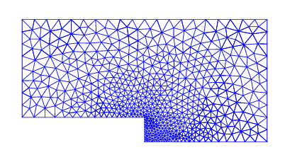
Fig. 6 Backwards facing step created using Gmsh
The height of the step is \(0.1L\). The height and width of the rectangular geometry is \(0.5L\) and \(L\) respectively. Use \(\mathrm{Re}=UL/\mu = 0.01\) (setting density to unity) as in Fig. 3-37 in [Whi06]. Set the velocity of the top (at \(y=0.5L\)) to constant \(\boldsymbol{u}=(1, 0)\). Use pseudo-traction for the inlet located at \(x=0\) and the outlet located at \(x=L\). No-slip for the bottom wall.
Create a suitable mesh using for example Gmsh. It is also possible to create this mesh directly using mshr.
4a) Compute the streamfunction. Note that you cannot use homogeneous Dirichlet on the entire domain for this case. Hint: enforce boundary conditions weakly. Use definition of the streamfunction (36) and n=FacetNormal(mesh) to implement the weak boundary form (second term on the left of second line in (48)).
4b) Make a contour plot, similar to Fig. 3-27 in [Whi06], of the streamfunction. Hint: Dump result to VTK-format and plot contours using paraview. To create a VTK-file for the streamfunction solution Function psi:
 f = File("psi.pvd")
 f << psi
4c) Compute the velocity flux in and out of the domain. Is mass being conserved? Hint: to compute the flow through left and right domains we need to integrate the solution over these domains only
Surface integrals like this can be computed in FEniCS by making use of SubDomains and a MeshFunction over the facets (the edges of the mesh):
def left(x, on_boundary):
       return x[0] < 1e-12 and on_boundary
Left = AutoSubDomain(left)
mf = MeshFunction("size_t", mesh, 1)
mf.set_all(0)
Left.mark(mf, 1)
ds = ds(subdomain_data=mf, domain=mesh)
Briefly, this code creates a Function that has an integer value on all facets (in 2D that means all the edges) in the mesh. The SubDomain Left is created by feeding an inside function (left) to the AutoSubDomain function. Left.mark(mf, 1) sets the value of all facets on the left boundary to 1. Using these tools we can now integrate over the left boundary exclusively. For example, to compute the area of the inlet do
A = assemble(Constant(1)*ds(1))
4d) Reverse the direction of the flow using \(\boldsymbol{u}=(-1, 0)\) for the top boundary. Does this change the streamlines? Explain the result.
4e) Compute the normal stress on the bottom wall. Is there any difference depending on the direction of the flow? Is this realistic for real flows of moderate Reynolds numbers?
The normal stress on the wall is computed as
where the stress tensor \(\tau = -p\boldsymbol{I}+\mu(\nabla \boldsymbol{u} + \nabla \boldsymbol{u}^T)\).