Demo - Integration of functions#
Mikael Mortensen (email: mikaem@math.uio.no), Department of Mathematics, University of Oslo.
Date: August 7, 2020
Summary. This is a demonstration of how the Python module shenfun can be used to integrate over 1D curves and 2D surfaces in 3D space. We make use of curvilinear coordinates, and reproduce some integrals performed by Behnam Hashemi with Chebfun.
Note
For all the examples below we could just as well use Legendre polynomials instead of Chebyshev. Just replace ‘C’ with ‘L’ when creating function spaces. The accuracy ought to be similar.
The inner product#
A lesser known fact about shenfun is that it can be used to perform regular, unweighted, integrals with spectral accuracy. With the newly added curvilinear coordinates feature, we can now also integrate over highly complex lines and surfaces embedded in a higher dimensional space.
To integrate over a domain in shenfun we use the inner() function, with a constant test function. The inner() function in shenfun is defined as an integral over the entire domain \(\Omega\) in question
for trial function \(u\), test function \(v\) and weight \(w\). Also, \(\overline{v}\) represents the complex conjugate of \(v\), in case we are working with complex functions (like Fourier exponentials).
The functions and weights take on different form, but if the test function \(v\) is chosen to be a constant, e.g., \(v=1\), then the weight is also constant, \(w=1\), and the inner product becomes an unweighted integral of \(u\) over the domain
Note that the integral in the inner product either can be computed exactly using Sympy, adaptively using Scipy or with quadrature using Shenfun. The quadrature can be computed with any fixed resolution, see inner().
Curve integrals#
For example, if we create some function space on the line from
0 to 1, then we can get the length of this domain using inner
from shenfun import *
B = FunctionSpace(10, 'C', domain=(0, 1))
u = Array(B, val=1)
length = inner(u, 1)
print('Length of domain =', length)
Note that we cannot simply do inner(1, 1), because the
inner function does not know about the domain, which is part
of the FunctionSpace. So to integrate u=1, we need to
create u as an Array with the constant value 1.
Since the function space B is Cartesian the computed
length is simply the domain length.
Not very impressive, but the same goes for multidimensional
tensor product domains
F = FunctionSpace(10, 'F', domain=(0, 2*np.pi))
T = TensorProductSpace(comm, (B, F))
area = inner(1, Array(T, val=1))
print('Area of domain =', area)
Still not very impressive, but moving to curvilinear coordinates it all starts to become more interesting. Lets look at a spiral \(C\) embedded in \(\mathbb{R}^3\), parametrized by one single parameter \(t\)
What is the length of this spiral? The spiral can be seen as the red curve in the figure a few cells below.
The integral over the parametrized curve \(C\) can be written as
We can find this integral easily using shenfun. Create a function space in curvilinear coordinates, providing the position vector \(\mathbf{r} = x(t)\mathbf{i} + y(t) \mathbf{j} + z(t) \mathbf{k}\) as input. Also, choose to work with covariant basis vectors, which is really not important unless you work with vector equations. The alternative is the default ‘normal’, where the basis vectors are normalized to unit length.
import sympy as sp
from shenfun import *
config['basisvectors'] = 'covariant'
t = sp.Symbol('x', real=True, positive=True)
rv = (sp.sin(2*t), sp.cos(2*t), 0.5*t)
C = FunctionSpace(100, 'C', domain=(0, 2*np.pi), coordinates=((t,), rv))
Then compute the arclength using inner(), again by using a constant testfunction 1, and a constant Array u=1
length = inner(1, Array(C, val=1))
print('Length of spiral =', length)
The arclength is found to be slightly longer than \(4 \pi\). Looking at the spiral below, the result looks reasonable.
%matplotlib inline

import matplotlib.pyplot as plt
fig = plt.figure(figsize=(4, 3))
X = C.cartesian_mesh(kind='uniform')
ax = fig.add_subplot(111, projection='3d')
p = ax.plot(X[0], X[1], X[2], 'r')
hx = ax.set_xticks(np.linspace(-1, 1, 5))
hy = ax.set_yticks(np.linspace(-1, 1, 5))
The term \(\sqrt{\left(\frac{d x}{d t}\right)^2 + \left(\frac{d y}{d t}\right)^2 + \left(\frac{d z}{d t}\right)^2}\) is actually here a constant \(\sqrt{4.25}\), found in shenfun as
C.coors.sg
We could also integrate a non-constant function over the spiral. For example, lets integrate the function \(f(x, y, z)= \sin^2 x\)
inner(1, Array(C, buffer=sp.sin(rv[0])**2))
which can be easily verified using, e.g., Wolfram Alpha
from IPython.display import IFrame
IFrame("https://www.wolframalpha.com/input/?i=integrate+sin%5E2%28sin%282t%29%29+sqrt%284.25%29+from+t%3D0+to+2pi", width="500px", height="350px")
Surface integrals#
Consider a 3D function \(f(x,y,z) \in \mathbb{R}^3\) and a 2D surface (not neccessarily plane) \(S(u, v)\), parametrized in two new coordinates \(u\) and \(v\). A position vector \(\mathbf{r}\) can be used to parametrize \(S\)
where \(\mathbf{i}, \mathbf{j}, \mathbf{k}\) are the Cartesian unit vectors. The two new coordinates \(u\) and \(v\) are functions of \(x, y, z\), and they each have a one-dimensional domain
The exact size of the domain depends on the problem at hand. The computational domain of the surface \(S\) is \(D=D_u \times D_v\).
A surface integral of \(f\) over \(S\) can now be written
where \(dS\) is a surface area element. With shenfun such integrals are trivial, even for highly complex domains.
Example 1#
Consider first the surface integral of \(f(x,y,z)=x^2\) over the unit sphere. We use regular spherical coordinates,
The straight forward implementation of a function space for the unit sphere reads
import sympy as sp

theta, phi = psi =sp.symbols('x,y', real=True, positive=True)
rv = (sp.sin(theta)*sp.cos(phi), sp.sin(theta)*sp.sin(phi), sp.cos(theta))

B0 = FunctionSpace(0, 'C', domain=(0, np.pi))
B1 = FunctionSpace(0, 'F', dtype='d')
T = TensorProductSpace(comm, (B0, B1), coordinates=(psi, rv, sp.Q.positive(sp.sin(theta))))
where sp.Q.positive(sp.sin(theta)) is a restriction that
helps Sympy in computing the Jacobian required for the integral.
We can now approximate the function \(f\) on this surface
f = Array(T, buffer=rv[0]**2)
and we can integrate over \(S\)
I = inner(1, f)
and finally compare to the exact result, which is \(4 \pi / 3\)
print('Error =', abs(I-4*np.pi/3))
Note that we can here achieve better accuracy by using
more quadrature points. For example by refining f
T = T.get_refined(2*np.array(f.global_shape))
f = Array(T, buffer=rv[0]**2)
print('Error =', abs(inner(1, f)-4*np.pi/3))
Not bad at all:-)
To go a little deeper into the integral, we can get the term \(\left|\frac{\partial \mathbf{r}}{\partial u} \times \frac{\partial \mathbf{r}}{\partial v} \right|\) as
print(T.coors.sg)
Here the printed variable is x, but this is because theta
is named x internally by Sympy. This is because of the definition
used above: theta, phi = sp.symbols('x,y', real=True, positive=True).
Note that \(\mathbf{b}_u = \frac{\partial \mathbf{r}}{\partial u}\) and
\(\mathbf{b}_v = \frac{\partial \mathbf{r}}{\partial v}\) are the two
basis vectors used by shenfun for the surface \(S\). The basis
vectors are obtainable as T.coors.b, and can also be printed
in latex using:
from IPython.display import Math
Math(T.coors.latex_basis_vectors(symbol_names={theta: '\\theta', phi: '\\phi'}))
where we tell latex to print theta as \(\theta\), and not x:-)
From the basis vectors it should be easy to see that \(\left| \mathbf{b}_{\theta} \times \mathbf{b}_{\phi} \right| = \sin \theta\).
Example 2#
Next, we solve Example 5 from the online resources at math24.net. Here
and the surface is defined by
with \(0 \le u \le 2, 0 \le v \le 2\pi\).
The implementation is only a few lines, and we end by comparing to the exact solution \(14 \pi /3\)
u, v = psi =sp.symbols('x,y', real=True, positive=True)
rv = (u*sp.cos(v), u*sp.sin(v), v)
B0 = FunctionSpace(0, 'C', domain=(0, 2))
B1 = FunctionSpace(0, 'C', domain=(0, np.pi))
T = TensorProductSpace(comm, (B0, B1), coordinates=(psi, rv))
f = Array(T, buffer=sp.sqrt(1+rv[0]**2+rv[1]**2))
print('Error =', abs(inner(1, f)-14*np.pi/3))
In this case the integral measure is
print(T.coors.sg)
Example 3#
In this third example we use a surface that looks like a seashell. Again, the example is taken from chebfun.
The surface of the seashell is parametrized with position vector
for \(0 \le u \le 2 \pi, -2 \pi \le v \le 2 \pi\).
The function \(f\) is now defined as
The implementation is
rv = (5*(1-v/(2*sp.pi))*sp.cos(2*v)*(1+sp.cos(u))/4 + sp.cos(2*v),
      5*(1-v/(2*sp.pi))*sp.sin(2*v)*(1+sp.cos(u))/4 + sp.sin(2*v),
      10*v/(2*sp.pi) + 5*(1-v/(2*sp.pi))*sp.sin(u)/4 + 15)

B0 = FunctionSpace(100, 'C', domain=(0, 2*np.pi))
B1 = FunctionSpace(100, 'C', domain=(-2*np.pi, 2*np.pi))
T = TensorProductSpace(comm, (B0, B1), coordinates=(psi, rv, sp.Q.positive(v-2*sp.pi)))

f = rv[0]+rv[1]+rv[2]
fb = Array(T, buffer=f)
I = inner(1, fb)
print(I)
which agrees very well with chebfun’s result. The basis vectors for the surface of the seashell are
Math(T.coors.latex_basis_vectors(symbol_names={u: 'u', v: 'v'}))
which, if nothing else, shows the power of symbolic computing in Sympy.
We can plot the seashell using either plotly or mayavi. Here we choose plotly since it integrates well with the executable jupyter book.
import plotly
fig = surf3D(fb, colorscale=plotly.colors.sequential.Jet)
fig.update_layout(scene_camera_eye=dict(x=1.6, y=-1.4, z=0))
fig.show()