Similarity solutions¶

Similarity solutions are obtained when the number of independent variables describing a problem is reduced by at least one.

Stokes’ first problem revisited¶

We will first illustrate this by revisiting Stokes’ first problem - A fluid initially at rest in an infinite domain (\(y\in[0, \infty)\)) is suddenly set in motion by an infinite flat plate located at \(y=0\). The problem is described by the equations

(35)¶\[\begin{split}\begin{aligned} \frac{\partial u}{\partial t} &= \nu \frac{\partial^2 u}{\partial y^2} \text{ for } y\in [0, \infty), \\ u(\infty, t) &= 0, \\ u(y, t<0) &= 0 \\ u(0, t>0) &= U_0 \end{aligned}\end{split}\]

We have already found the solution to this problem using Fourier integrals with the solution as shown below

import numpy as np
from scipy.special import erf
import matplotlib.pyplot as plt
%matplotlib inline

nu = 0.01
U0 = 1.
y = np.linspace(0.01, 10, 100)
plt.figure(figsize=(6, 4))
for i in range(1, 10):
    t = i * 200.
    u = U0*(1-erf(y/2/np.sqrt(nu*t)))
    plt.plot(u, y, "k")    
plt.annotate(r'Time', xy=(0.5, 4.6),
             xytext=(-80, -90), textcoords='offset points', 
             arrowprops=dict(arrowstyle="->", connectionstyle="arc3,rad=-.15"))
plt.xlabel("Velocity " + r"$u/U_0$")
plt.ylabel("Position " + "$y$")
plt.title("Stokes' first problem")
plt.show()

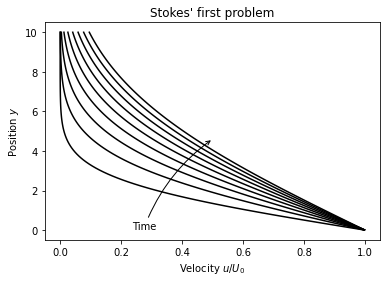
The solution is repeated here

\[ u(y, t) = U_0\left(1-\mathrm{erf} \left(\frac{y}{2\sqrt{\nu t}} \right) \right).\]

We will now look at this problem again and try to find this solution using a similarity approach. First define a similarity variable

\[ \eta = \frac{y}{2 \sqrt{\nu t}},\]

and observe that the solution can be written in terms of merely one variable

\[ u(\eta) = U_0\left(1-\mathrm{erf} (\eta) \right).\]

Usually we don’t know the solution and have to guess a similarity variable. Having defined \(\eta\), the heat equation (35) can be rewritten using chain rule differentiation

\[ \frac{\mathrm{d} u}{\mathrm{d} \eta} \frac{\partial \eta}{\partial t} - \nu \left( \frac{\mathrm{d}^2 u}{\mathrm{d} \eta^2} \left( \frac{\partial \eta}{\partial y} \right)^2 + \frac{\mathrm{d} u}{\mathrm{d} \eta} \frac{\partial^2 \eta}{\partial y^2} \right) = 0.\]

The partial derivatives of \(\eta\) are

\[\begin{split}\begin{aligned} \frac{\partial \eta}{\partial t} &= -\frac{\eta}{2 t}, \\ \frac{\partial \eta}{\partial y} &= \frac{1}{2\sqrt{\nu t}}, \\ \frac{\partial^2 \eta}{\partial y^2} &= 0. \end{aligned}\end{split}\]

Inserting this into the above leads to and ordinary differential equation for \(u(\eta)\), which is exactly what we were hoping to achieve

\[ 2\eta \frac{\mathrm{d} u}{\mathrm{d} \eta} + \frac{\mathrm{d}^2 u}{\mathrm{d} \eta^2} = 0.\]

This ordinary differential equation must be solved using boundary conditions \(u(0) = U_0\) and \(u(\infty) = 0\). Define first \(h(\eta) = \mathrm{d} u / \mathrm{d}\eta\) and rewrite the ODE as

\[ 2\eta h + \frac{\mathrm{d} h}{\mathrm{d} \eta} = 0.\]

Separate variables and integrate to obtain

\[ \frac{\mathrm{d} u}{\mathrm{d} \eta} = Ae ^{- \eta^2}.\]

Integrate one more time to obtain

\[ u(\eta) = A\mathrm{erf} (\eta) + B\]

Inserting for the boundary conditions we finally get the original solution derived with much more effort in Unsteady Couette flows.

Plane stagnation flow¶

Another well known and much used similarity solution is the streamfunction \(\psi(\boldsymbol{x}, t)\), that is most often used for two-dimensional flows, where it is defined through

(36)¶\[ u = \frac{\partial \psi}{\partial y}, \quad v = -\frac{\partial \psi}{\partial x}.\]

In 2D the only non-zero component of the vorticity vector, \(\omega_z\), is computed as

\[ \omega_z = \frac{\partial v}{\partial x} - \frac{\partial u}{\partial y},\]

If this definition is combined with (36) we obtain a Poisson equation for the streamfunction

(37)¶\[ \nabla^2 \psi = -\omega_z.\]

The streamfunction is much used for inviscid irrotational flows, where the vorticity component \(\omega_z=0\). However, the definition of the streamfunction is equally valid for viscous flows.

An illustration of plane stagnation flow is given in Fig. (3-24) of [Whi06]. For inviscid flows the solution is trivially obtained as

\[\psi = Bxy, \quad u = Bx, \quad v = -By,\]

where \(B\) is a positive constant. Make sure to check that the solution satisfies both (37) (with zero right hand side) and the continuity equation

\[ \frac{\partial u}{\partial x} + \frac{\partial v}{\partial y} = 0.\]

For viscous flows it is somewhat more complicated, since the right hand side of (37) is nonzero. To find the solution for viscous flows we also need to consider the momentum equations in two dimensions

(38)¶\[\begin{split}\begin{aligned} \underline{u\frac{\partial u}{\partial x}} + v\frac{\partial u}{\partial y} &= -\frac{1}{\rho}\frac{\partial p}{\partial x} + \nu \left(\frac{\partial^2 u}{\partial x^2} + \frac{\partial^2 u}{\partial y^2} \right), \notag \\ u\frac{\partial v}{\partial x} + \underline{v\frac{\partial v}{\partial y}} &= -\frac{1}{\rho}\frac{\partial p}{\partial y} + \nu \left(\frac{\partial^2 v}{\partial x^2} + \frac{\partial^2 v}{\partial y^2} \right). \end{aligned}\end{split}\]

These equations are nonlinear due to the two underlined terms and coupled through the continuity equation. Note that there are three equations for the three unknowns \(u, v, p\), so the equations are closed. We will now look for a similarity solution through a modification of the streamfunction of the form

\[ \psi_{\nu} = B x f(y), \quad u = \frac{\partial \psi_{\nu}}{\partial y} = Bx \frac{d f}{dy}, \quad v = -\frac{\partial \psi_{\nu}}{\partial x} = -Bf.\]

Using an apostrophe for the derivative of \(f\) with respect to \(y\) one has immediately

\[\begin{split}\begin{aligned} \frac{\partial u}{\partial x} = B f^{\prime},\quad \frac{\partial u}{\partial y} = Bx f^{\prime\prime}, \quad \frac{\partial^2 u}{\partial x^2} = 0,\quad \frac{\partial^2 u}{\partial y^2} = Bx f^{\prime\prime\prime}, \\ \frac{\partial v}{\partial x} = 0,\quad \frac{\partial v}{\partial y} = -B f^{\prime}, \quad \frac{\partial^2 v}{\partial x^2} = 0,\quad \frac{\partial^2 v}{\partial y^2} = -B f^{\prime\prime}. \end{aligned}\end{split}\]

We immediately see that the continuity equation is satisfied. Inserting for the streamfunction in (38) we obtain

\[\begin{split}\begin{aligned} B^2 x (f^{\prime})^2 - B^2 x f f^{\prime\prime} - \nu B x f^{\prime\prime\prime} = -\frac{1}{\rho} \frac{\partial p}{\partial x}, \\ B^2 f f^{\prime} + \nu B f^{\prime\prime} = -\frac{1}{\rho} \frac{\partial p}{\partial y} \end{aligned}\end{split}\]

The last equation here states that \(\partial p/\partial y\) is only a function of \(y\) and thus

(39)¶\[ \frac{\partial^2 p}{\partial x \partial y} = 0.\]

The momentum equation in the \(x\)-direction can be simplified by dividing through by \(- \nu B x\)

(40)¶\[ f^{\prime\prime\prime} + \frac{B}{\nu} \left( f f^{\prime\prime} - (f^{\prime})^2\right) = \frac{1}{\nu B x \rho} \frac{\partial p}{\partial x}\]

The left hand side is only a function of \(y\) and as such we need the right hand side also as a function of only \(y\). For this to happen it is evident that the pressure derivative \(\partial p / \partial x = \mathrm{const} \, x \, h(y)\), where \(h(y)\) is some function of \(y\). However, from Eq. (39) it follows that \(h\) must be a constant as well and as such the right hand side of (40) must be constant. Since the right hand side is constant, this means that the left hand side also must be a constant.

Treating the right hand side as a constant we can compute its value using the boundary conditions \(f^{\prime}=1, f^{\prime \prime}=f^{\prime\prime\prime}=0\) for \(y\longrightarrow \infty\) (the first follows from freestream condition \(u_{viscous}=u_{inviscid}\)). Inserted for the boundary conditions we obtain finally

(41)¶\[ f^{\prime\prime\prime} + \frac{B}{\nu} \left( f f^{\prime\prime} - (f^{\prime})^2\right) =- \frac{B}{\nu}.\]

Note that (41) is an exact equation for stagnation flow, since no terms have been eliminated in its derivation. The equation is nonlinear, which calls for iterative numerical solution techniques. The equation can be non-dimensionalised using length- and velocity-scales \(\sqrt{\nu/B}\) and \(\sqrt{\nu B}\) respectively, and the dimensionless variables

(42)¶\[ \eta = y \sqrt{\frac{B}{\nu}}, \quad \psi = x F(\eta) \sqrt{B\nu}.\]

We can now easily obtain

\[\begin{split}\begin{aligned} f(y) &= F\sqrt{\frac{\nu}{B}}, \\ f^{\prime} &= \frac{dF}{d\eta}\frac{d\eta}{dy} \sqrt{\frac{\nu}{B}} = F^{\prime} \sqrt{\frac{B}{\nu}} \sqrt{\frac{\nu}{B}} = F^{\prime}, \\ f^{\prime\prime} &= \frac{dF^{\prime}}{d\eta}\frac{d\eta}{dy} = F^{\prime\prime}\sqrt{\frac{B}{\nu}}, \\ f^{\prime\prime\prime} &= \frac{dF^{\prime\prime}}{d\eta}\frac{d\eta}{dy} = F^{\prime\prime\prime}\frac{B}{\nu}. \end{aligned}\end{split}\]

Inserted into (41) we obtain the dimensionless equation

(43)¶\[ F^{\prime\prime\prime} + F F^{\prime\prime} + 1 - (F^{\prime})^2 = 0,\]

that can be solved using boundary conditions \(F(0)=F^{\prime}(0)=0\) and \(F^{\prime}(\infty)=1\).

Axisymmetric stagnation flow¶

The plane stagnation flow discussed in the previous section is stagnant for a line in the \(z\)-plane located at \(x=0\). Axisymmetric stagnation flow is similar in form, but only stagnant in a single point located at \(x=y=z=0\). This axisymmetric flow is what you obtain by pointing a garden hose directly towards a plane wall (neglecting gravity). The equations are similar to the plane flow, but may be simplified using cylindrical coordinates. A streamfunction in cylindrical coordinates can be defined through

(44)¶\[ u_{r} = -\frac{1}{r}\frac{\partial \psi}{\partial z}, \quad u_{z} = \frac{1}{r}\frac{\partial \psi}{\partial r}\]

For axisymmetric flows with \(u_{\theta}=0\) the continuity equation reads

\[ \frac{1}{r}\frac{\partial r u_r}{\partial r} + \frac{\partial u_z}{\partial z} = 0.\]

Inserting for (44) it is easily verified that continuity is satisfied.

The streamfunction for axisymmetric inviscid flow towards a stagnation point is given as

\[ \psi = -B r^2 z\]

which leads to velocity components

\[ u_r = B r, \quad u_z = -2B z\]

For viscous flows one may obtain a dimensionless similarity solution using

\[ \psi = - r^2 F(\eta) \sqrt{B \nu}, \quad \eta = z\sqrt{\frac{B}{\nu}}.\]

Inserting into the momentum equation for \(u_{r}\) the mathematics are very much like in the previous section leading to

(45)¶\[ F^{\prime\prime\prime} + 2 F F^{\prime\prime} + 1 - (F^{\prime})^2 = 0.\]

This differs from plane stagnation flow only by the factor 2.

MEK4300 Lecture notes

Similarity solutions¶

Stokes’ first problem revisited¶

Plane stagnation flow¶

Axisymmetric stagnation flow¶

Suggested assignments similarity solutions¶