Suggested solutions Couette
Solutions written assignments Couette
Problem 3-1 in White
Solve for a non-Newtonian Couette flow, where the stress tensor is computed as
where \(n\) is an integer different from 1. The momentum equation for any stress tensor in a Couette flow is
For one-dimensional Couette flow aligned with the \(x\)-direction and homogeneous in the \(z\)-direction, the equation reads
which means that \(\tau\) is a constant with respect to \(y\) and thus
where \(K_2\) is a new constant. In other words
and thus
The solution is the same as for Newtonian flows regardless of \(n\).
Problem 3-2 in White
The analytical solution has already been computed in Eq. (10) in Couette flows.
Problem 3-3 in White
The temperature equation reduces to
Inserting for Eq. (10) we have
Integrate twice to obtain
and determine constants using the two boundary conditions.
Problem 3-4 in White
The problem reads: solve the Laplace equation in cylindrical coordinates (8) with boundary conditions \(u(0)=U\) and \(u(\infty)=0\). The solution for the velocity is given in Eq. (9) and inserted for the boundary conditions we need to find \(C_1\) and \(C_2\) such that
The first condition requires \(C_1=0\) and thus \(C_2=U\). The second condition requires \(C_2=0\), which is a contradiction. It is not possible to satisfy both boundary conditions. Physically, the boundary layer that is being dragged by the rod will continue to grow indefinitely and there is no steady state solution possible for this problem.
Problem 3-5 in White
Solve the momentum equation for the angular velocity
with boundary conditions \(u(R)=\omega R\) and \(u(\infty)=0\). The solution to this equation is given by [Whi06]
The boundary conditions are then
which leads to \(C_1=0\) and \(C_2=\omega R^2\) and thus the angular velocity
which agrees with the solution of a potential vortex. The pressure is found from the r-momentum equation
which can be integrated to
and where the constant can be found by assuming \(p(R)=p_0\) such that
which is what we would find using Bernoulli’s equation for a potential vortex (\(p_0+0.5\rho (\omega R)^2 = p + 0.5 \rho u^2\)).
Homogeneous heat equation with inhomogeneous boundary conditions
We consider the additional problem Homogeneous heat equation with inhomogeneous boundary conditions.
Introducing the function \(\boldsymbol{U}(y, t) = 1/L[(L-y)g(t) + y h(t)]\) and \(v(y, t) = u(y, t) - \boldsymbol{U}(y, t)\) we obtain an inhomogeneous heat equation with homogeneous boundary conditions as given in Hint 2. The right hand side function, boundary conditions and initial conditions can be found straight forward as
The solution to the homogeneous part of the problem can be found using separation of variables \(v^h(y, t) = T(t) V(y)\)
and thus \(T(t) = e^{-\lambda^2 \nu t}\). The boundary conditions give \(V(y) = A \sin(\lambda y)\) and to satisfy initial conditions we need to use superposition and a range of solutions. The homogeneous solution thus reads
where we can find \(A_n\) using the initial condition and orthogonality, i.e., multiply \(v^h(y,0)(=\overline{\phi}(y))\) by \(\sin(\lambda_m y)\) and integrate to obtain
where the last step follows if \(\overline{\phi}(y)\) is an odd function. The solution to the inhomogeneous part of the problem reuses the homogeneous solution, but replaces \(\overline{\phi}(y)\) with \(f(y,s)\) when computing the coefficients. We thus replace \(A_n\) with \(B_n(t)\) and compute it as
Using superposition in time the inhomogeneous solution is thus
and the general solution to our original problem is
Specific solution where \(g(t) = U_0 \cos (\omega t)\), \(h(t)=0\) and \(\phi(y)=U_0(1-y/L)\). The problem now reads for \(v(y,t) = u(y, t) - \boldsymbol{U}(y, t)\)
\[\begin{split} \begin{aligned} \frac{\partial v}{\partial t} - \nu \frac{\partial ^2 v}{\partial y^2} &= f(y, t) = U_0 \omega (1-\frac{y}{L}) \sin(\omega t) , \quad \mathrm{ for }\quad 0 \leq y \leq L \\ \notag v(y, 0) &= U_0(1-\frac{y}{L}) - U_0(1- \frac{y}{L}) = 0, \\ \notag v(0, t) &= v(L, t) = 0, \end{aligned} \end{split}\]and naturally the homogeneous solution is identically zero, i.e., \(v^h(y, t) = 0\). The inhomogeneous contribution to the total solution is found by computing \(B_n\) and \(v^p\). Both integrals can be obtained using Wolfram alpha, the first one reads
\[\begin{split} \begin{aligned} B_n(t) &= \frac{2}{L} \int_0^L \sin(\lambda_n y) U_0 \omega (1-\frac{y}{L}) \sin(\omega t) \mathrm{d}y, \\ &= \frac{2 U_0 \omega \sin(\omega t)}{\lambda_n L}. \end{aligned} \end{split}\]Inserted into the equation for \(v^p\) one obtains
\[ v^p(y, t) = \frac{2 U_0 \omega }{L} \int_0^t \sum_{n=1}^{\infty} \frac{\sin(\lambda_n y)}{\lambda_n} e^{-\lambda_n^2 \nu (t-s)}\sin(\omega s) \mathrm{d}s, \]which Wolfram alpha tells me is equal to
\[ v^p(y, t) = \frac{2 U_0 \omega }{L} \sum\limits_{n=1}^{\infty} \frac{\sin(\lambda_n y)}{\lambda_n} \left(\frac{\nu\lambda_n^2\sin(\omega t)-\omega\cos(\omega t) + \omega e^{-\lambda_n^2\nu t}}{\omega^2 + \lambda_n^4\nu^2}\right). \]The total solution is thus \(u(y, t) = v^p(y,t) + U_0\cos(\omega t) (1-y/L)\).
Flow between rotating concentric cylinders
"""
Flow between rotating concentric cylinders
"""
from dolfin import *
import matplotlib.pyplot as plt
%matplotlib inline
r0, r1 = 0.2, 1
mesh = IntervalMesh(100, r0, r1)
V = FunctionSpace(mesh, 'CG', 1)
u = TrialFunction(V)
v = TestFunction(V)
x = Expression("x[0]", degree=1)
w0, w1 = Constant(1.), Constant(0.1)
T0, T1 = Constant(8), Constant(10)
mu = Constant(0.25)
k = Constant(0.001)
u_ = Function(V)
T_ = Function(V)
F = inner(grad(v), grad(u))*x*dx + u*v/x*dx
FT = inner(grad(v), grad(u))*x*dx - mu/k*v*x*(u_.dx(0)-u_/x)**2*dx
def inner_bnd(x, on_bnd):
return on_bnd and x[0] < r0+DOLFIN_EPS
def outer_bnd(x, on_bnd):
return on_bnd and x[0] > 1-DOLFIN_EPS
bci = DirichletBC(V, r0*w0(0), "std::abs(x[0]-{}) < 1.e-12".format(r0))
bco = DirichletBC(V, r1*w1, outer_bnd)
bcTi = DirichletBC(V, T0, inner_bnd)
bcTo = DirichletBC(V, T1, outer_bnd)
solve(lhs(F) == rhs(F), u_, bcs=[bci, bco])
solve(lhs(FT) == rhs(FT), T_, bcs=[bcTi, bcTo])
# Compute exact solution given in (3.22)
ue = project(r0*w0*(r1/x-x/r1)/(r1/r0-r0/r1) +
r1*w1*(x/r0-r0/x)/(r1/r0-r0/r1), V)
# Compute exact solution given in (3.23)
Tn = project((T_-T0)/(T1-T0), V)
PrEc = mu*r0**2*w0**2/k/(T1-T0)
Te = PrEc*r1**4/(r1**2-r0**2)**2*((1-r0**2/x**2) - (1-r0**2/r1**2)*ln(x/r0)/ln(r1/r0)) + ln(x/r0)/ln(r1/r0)
Te = project(Te, V)
print("\nError velocity = ", errornorm(u_, ue, degree_rise=0))
print("Error temperature = ", errornorm(Tn, Te, degree_rise=0))
print("??? Should be close to zero.\n")
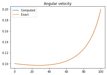
plt.figure()
plt.plot(u_.vector().get_local())
plt.plot(ue.vector().get_local())
plt.title("Angular velocity")
plt.legend(('Computed', 'Exact'))
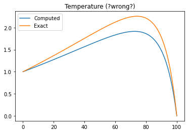
plt.figure()
plt.plot(Tn.vector().get_local())
plt.plot(Te.vector().get_local())
plt.title("Temperature (?wrong?)")
plt.legend(('Computed', 'Exact'))
# Since I cannot reproduce the temperature I have recomputed
# (3.23) analytically. I plot that result here
C1 = w0-r1**2*(w1-w0)/(r0**2-r1**2)
C2 = r1**2*(w1-w0)/(1-r1**2/r0**2)
C3 = (T1-T0+C2**2*mu/k*(1/r1**2-1/r0**2))/ln(r1/r0)
C4 = T0 + C2**2*mu/k/r0**2-C3*ln(r0)
Tee = project((-C2**2*mu/k/x**2+C3*ln(x)+C4-T0)/(T1-T0), V)
print("\nError recomputed temperature = ", errornorm(Tn, Tee))
print("Which is a strong indication that (3.23) is wrong!!")
plt.show()
Error velocity    =  1.1540847636407312e-05
Error temperature =  0.20666794167009878
??? Should be close to zero.


Error recomputed temperature =  0.000492714248321644
Which is a strong indication that (3.23) is wrong!!